

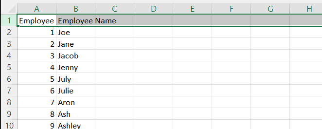
In this course, I will cover the basics of Excel, which will help you make a good first impression. No matter how little experience you have in Excel, I assure you that by reading this blog, you will understand Excel features and how to use them. Once you grasp the concepts outlined here, you will begin using Excel effectively. One thing I want to emphasize is not to be intimidated by Excel. You can do it! Regardless of which version of Excel you have, this blog is all you need to get started.
I ask for two things from you: your full attention and a commitment to apply what is mentioned here by actively engaging with the material. This is because we know that simply reading or listening isn’t enough for effective learning and retention, I ask for your commitment to actively engage with the material. Promise me you’ll learn by doing.
We’ll learn how to create and save workbooks, as well as the basics of spreadsheet anatomy, layouts, and how it works. This knowledge will help you use it effectively for various projects or tasks.


Let’s get started
I have divided this informative blog into different sections, each providing useful information that you can use to start your Excel journey and make a good first impression.
1) Anatomy Of Excel
So, let’s get started with understanding the different basic features of Excel, which will improve your familiarity with the software.
So, whenever you open Excel, it will take you to a similar screen. Here, I am using the online free version. If you haven’t used Excel before, no recent spreadsheets or workbooks will show under the ‘ recent or recently opened’ heading.
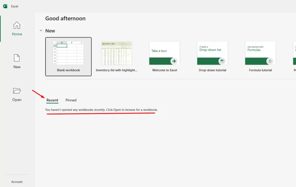
You can create a new blank workbook by clicking on the ‘Blank Workbook’ button at the top and start using the software, adding your data to your first or new project.
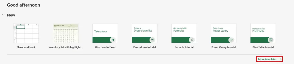
There are templates available that you can select, which will make your work more efficient since everything in those templates is predefined, from styling to headings to formulas. You can open templates by clicking on the ‘More templates →’ on the right side of the screen.
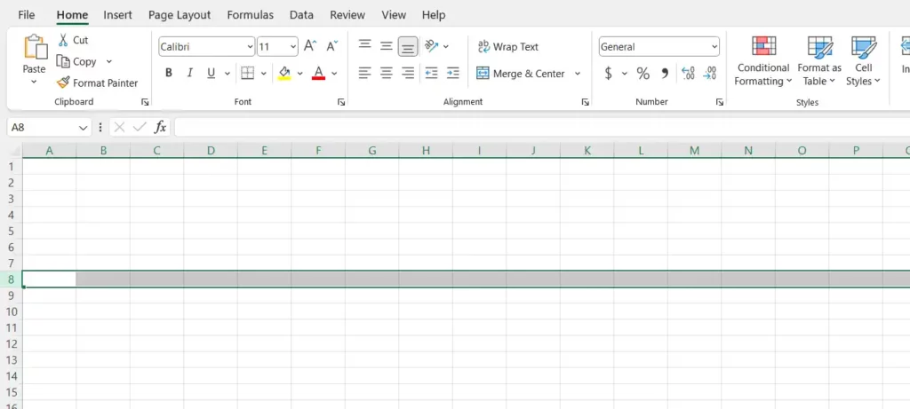
But I am going to click on the ‘Blank Workbook’ to open a completely empty workbook in Microsoft Excel so that I can teach you how to use the software. Before we start creating anything in the workbook, let’s discuss the anatomy of the spreadsheet. When you open the workbook, you start with one sheet, which you can see at the bottom-left corner of the screen. There is a possibility that you may have multiple sheets when you open a template, and all these sheets together are called a workbook.
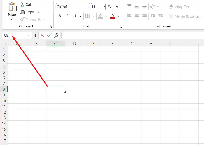
Similarly, we also have rows in the spreadsheet: 1, 2, 3, 4, 5, and so on. When you click on a row, the entire row gets selected. For example, in the screenshot, you can see that I clicked on row 8, and the entire row was selected.
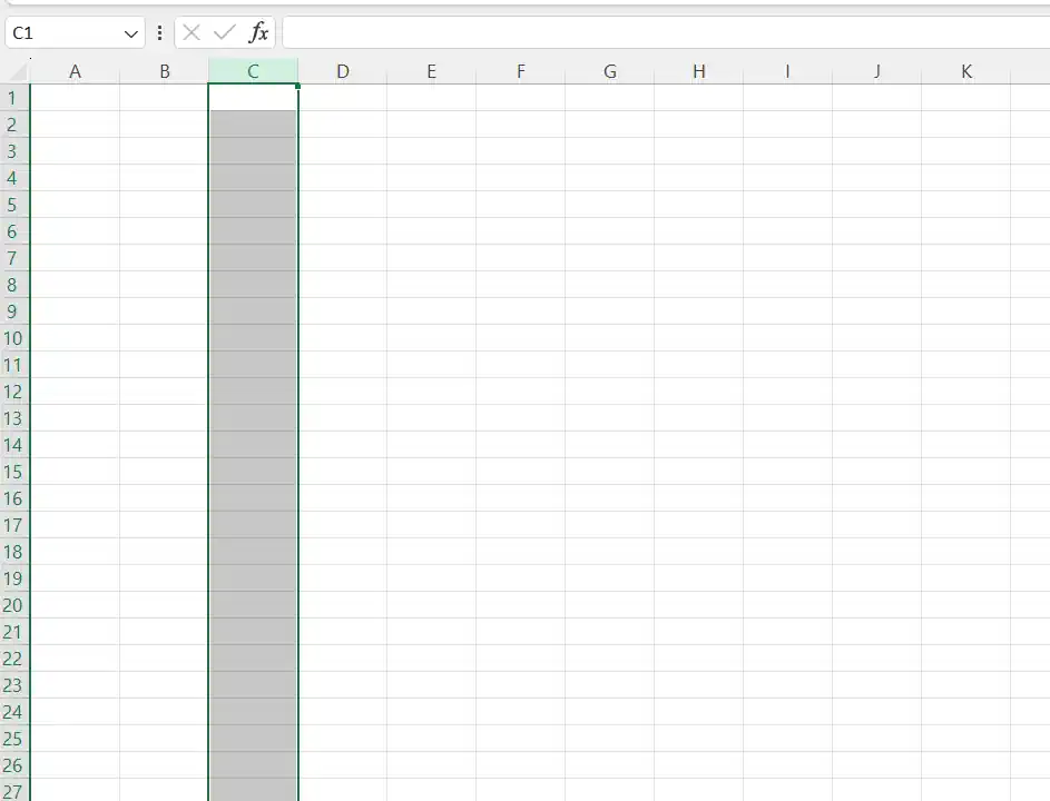
Like rows, spreadsheets also consist of columns labeled with letters such as A, B, C, D, E, F, G, and so on. To select an entire column, just click on the column’s letter, and it will be selected automatically. For example, in the screenshot, you can see that I clicked on row C, and the entire row was selected.
Every row has a number and every column has a letter, and the intersection of a row and column is what we call a cell. For example, in the screenshot, the cell C8 is the intersection of column C and row 8. There are 17 billion cells in total. When you click on a column, it becomes the active cell, and every cell is unique, which makes it powerful. This ensures that there won’t be any ambiguity as you work in Excel. You’ll come to appreciate this feature more as you learn and use Excel more frequently.
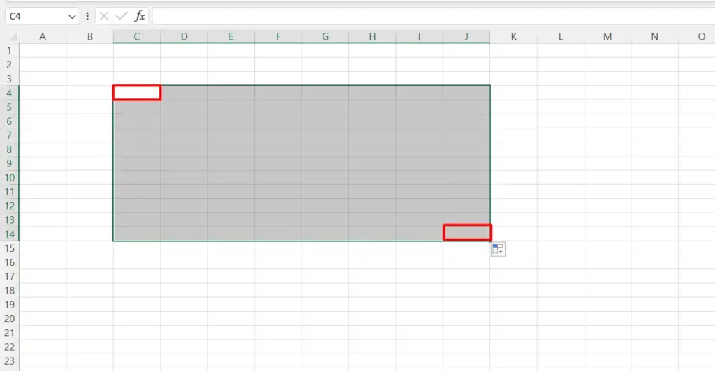
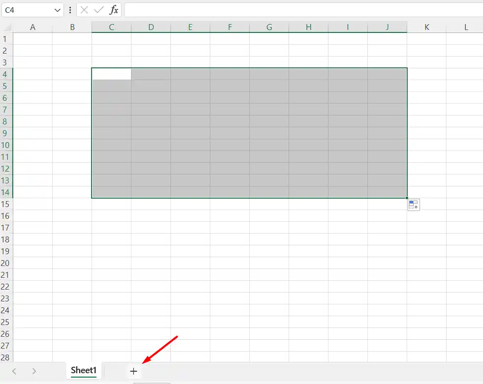
The next part of the anatomy of Excel is the range, which is a collection of cells generally grouped together. To create a range, you have to click and drag; once you stop, it becomes the range. For example, in the screenshot, I clicked on cell C4 and stopped at J14. The description of this range is from cell C4 through J14 or C4:J14, and in Excel, you express this with a colon (:). This is very important, and you will learn more about it as you start using Excel more and more.
You can add more worksheets by clicking on the plus sign next to the sheet and keep adding according to your requirements. After adding a new worksheet to the workbook, you can input data. As you advance, you’ll learn to make the data in these sheets interact with each other using formulas and functions.
In Excel, there are multiple tabs at the top, each offering different tools for your use. When you click on a tab, the tool buttons change, and all the tools are displayed in the layout called the ribbon. The tools in the ribbon are further divided into groups, and each group of tools is separated by a line, as you can see in the screenshot above. Sometimes there is a launch button because not all functionality can be shown in the ribbon.
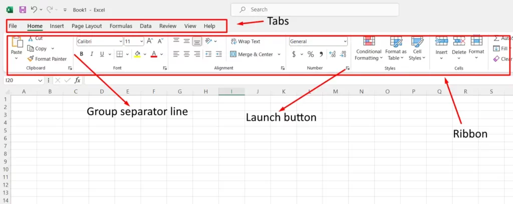
When you click on the launch button then it will open up even more options that can normally fit in the space provided in the ribbon.
Other than these things, there are other features or parts of the anatomy of the spreadsheet, such as the scroll bar on the right-hand side, which you can use to scroll up or down your spreadsheet. We also have a horizontal scroll bar, which you can use to move your spreadsheet from right to left or left to right. Additionally, there is a zoom option underneath the horizontal scroll bar.
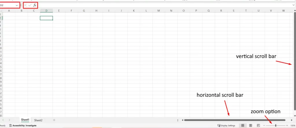
We also have the name box, which will display the name of the active cell or range, or provide a description. Next to it, there is the formula box, which you can use to add formulas to the data you have entered. On top of that, there is quick access to different functionalities that you can edit and include the most common features you think you will be using. This will improve the workflow and enhance your Excel experience. There are undo and redo buttons at the top, which will be very useful once you start using them.
2) Entering Data into the Spreadsheet
Let’s learn how to add data to the spreadsheet and arrange it so that you can perform calculations and make sense of your data.
So, whenever you want to add data to the spreadsheet, you have to select the cell and then tap Enter to enter the data inside the cell. When you press Enter, you move to the next cell, and it becomes active.
Autofill Handle
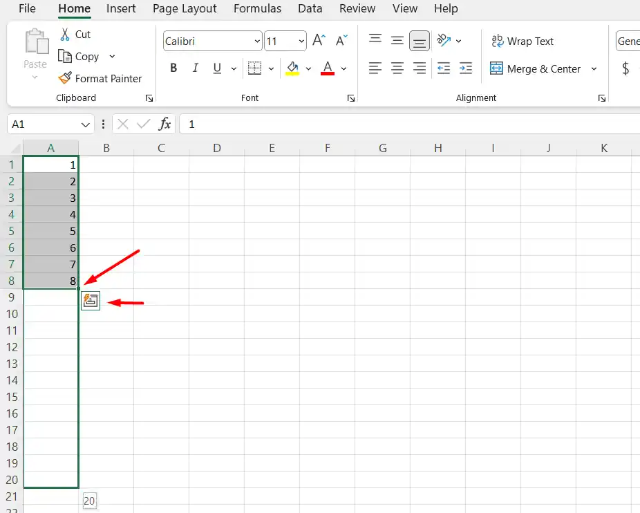
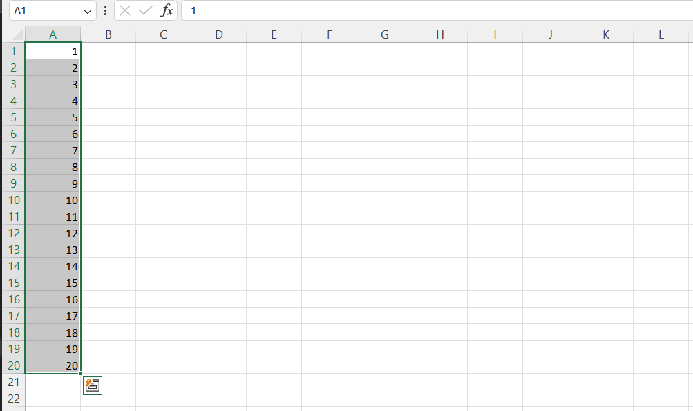
If the data you are adding to the spreadsheet follows a common pattern, you can utilize Excel’s built-in automatic functionality and use the autofill handle feature. To do this, you manually enter the data, select the cells, and once Excel identifies the pattern, you will see the autofill icon. You can then use this to speed up and automate repetitive tasks.
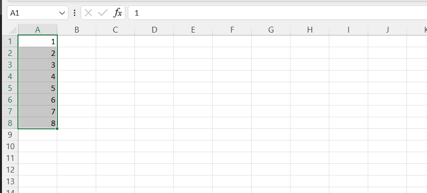
To autofill the data, place your cursor on the green dot until it becomes a black plus sign in color.
Double vs Single click on cell in Excel
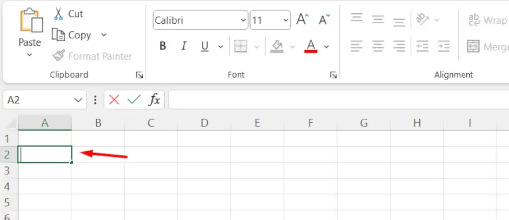
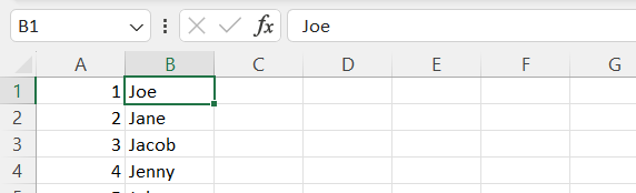
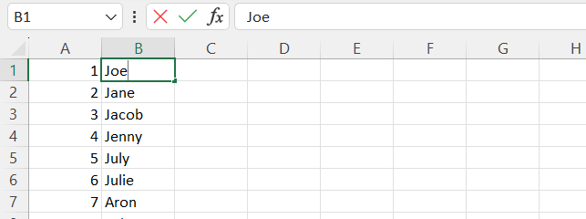
You can enter other data such as names, and one important thing: when you click on the cell, the whole cell is selected. If you write something, then whatever you’ve written in the cell will be erased. So, make sure you double-click on the cell if you want to change what you’ve written inside it.
Single click
Double click
Essential Spreadsheet Navigation and Shortcuts
You can use arrow keys to move up and down, left and right; Tab keys to move right, and Shift+Tab to move left; Enter to move down, and Shift+Enter to move up in the cell. You can copy and paste using Ctrl+C and Ctrl+V, which is a very easy and faster way to do it. You can also delete the data by selecting the ‘Clear All’ tool from the ribbon. You can use Ctrl+X to cut and move data from one cell or range to another, or you can select the cell and range, then press the mouse button and move the data wherever you want it to go.
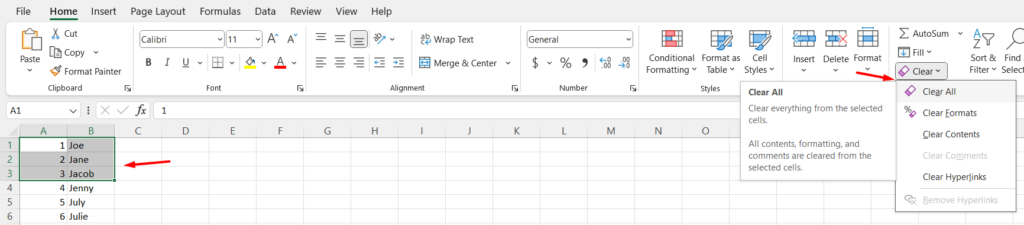
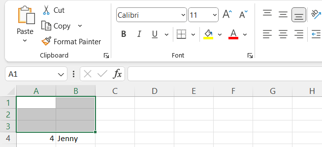
After clicking on clear all
Adding Blank Rows or Columns in Excel
To add a blank row or column in Excel, first select the row or column where you want to insert the blank space. You can do this by clicking on the row number or column letter to highlight it. Then, right-click on the selected row or column to bring up a context menu. From the options in the context menu, choose “Insert.” This command tells Excel to insert a new row above the selected row or a new column to the left of the selected column. After selecting “Insert,” Excel will add a new blank row above the chosen row or a blank column to the left of the selected column. This straightforward process allows you to easily insert blank rows or columns as needed, helping you organize and structure your data effectively within your Excel spreadsheet.
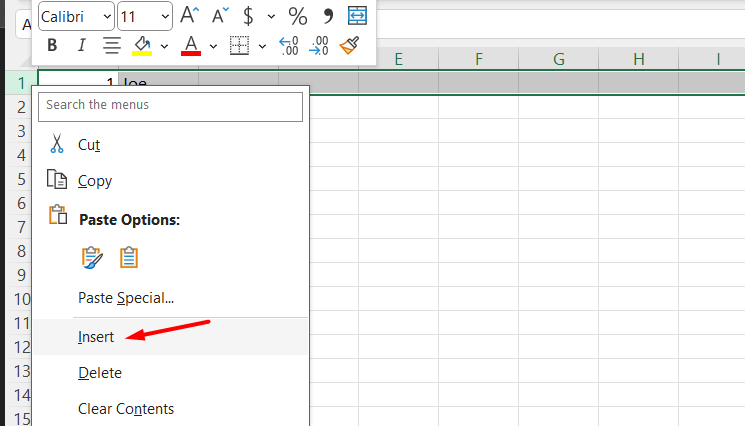
After clicking on insert
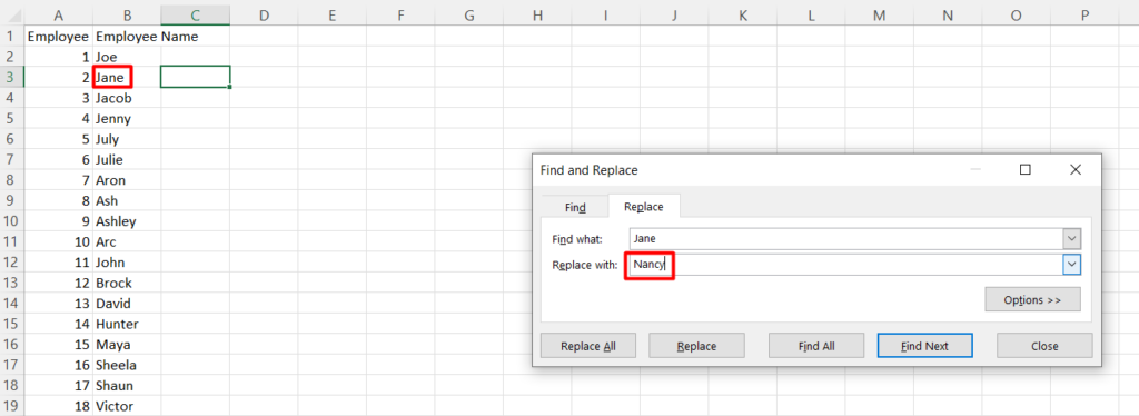
Change data in Excel
If you want to change data that you wrongly added and replace it with correct data, you can use the find and replace tool. You will find it on the right side of the ribbon. Click on the magnifying glass icon, then select the replace option, or you can press CTRL+H, which is a faster way to access the find and replace option. A pop-up will open in which you have to add the value you want to replace and then the value that you want to replace it with.
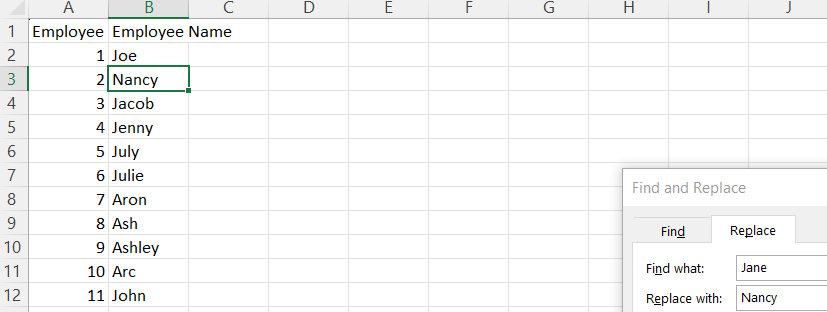
After pressing the replace button
3) Formulas in Excel
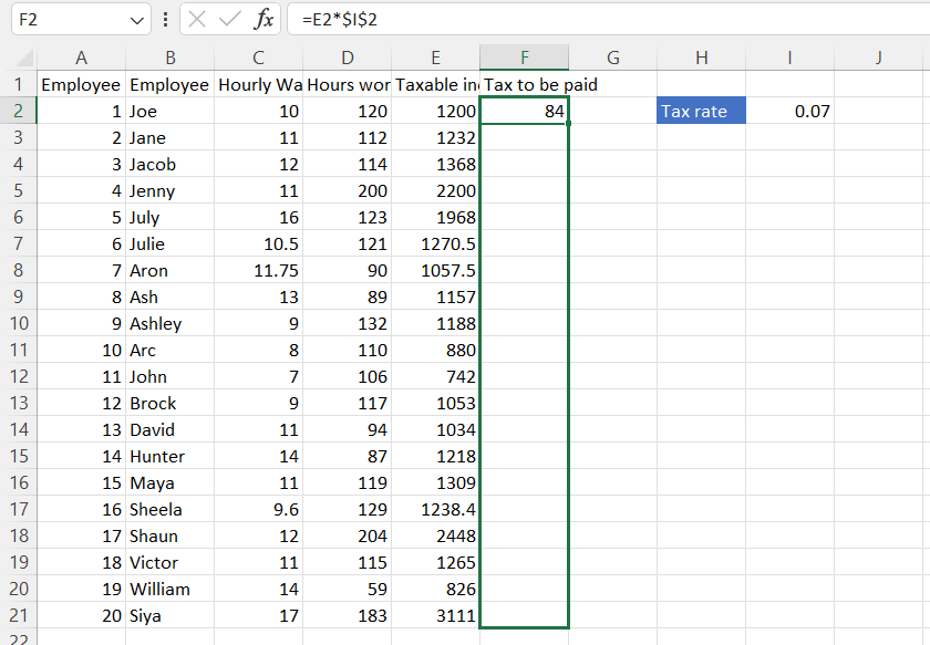
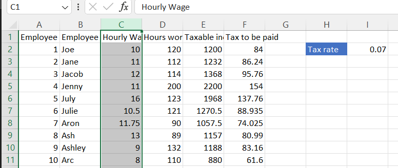
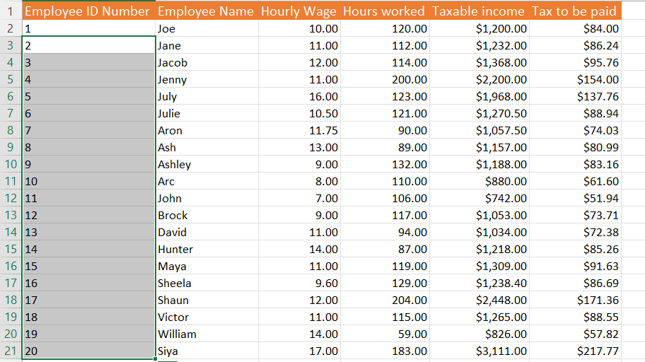
In Excel, you have access to various formulas that facilitate calculations, including addition (+), subtraction (-), multiplication (*), and division (/). Let’s explore some of these basic formulas together. Before performing calculations, let’s add data related to salary.
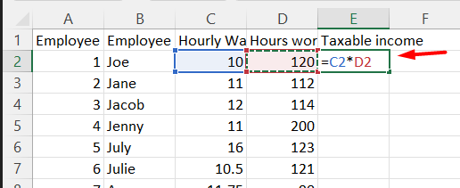
Imagine you need to calculate Joe’s total salary. To do this, start by entering the equal sign (=) in a new cell. Then, select the cell containing Joe’s hourly wage, followed by typing the asterisk symbol (*) for multiplication. After that, select the cell containing the number of hours worked by Joe. Finally, press Enter, and Excel will automatically compute the total salary.
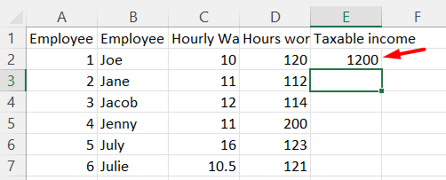
It’s important to note that this formula is dynamic, meaning that if you make any changes to the data (such as updating the hourly wage or hours worked), Excel will adjust the total salary accordingly. This dynamic nature ensures that your calculations remain accurate and up-to-date as your data changes.
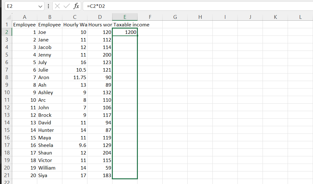
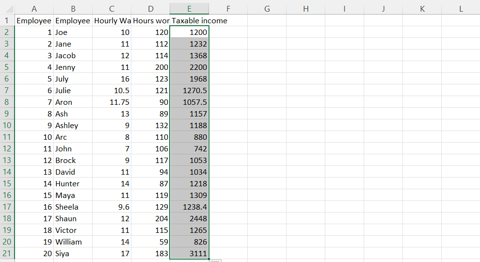
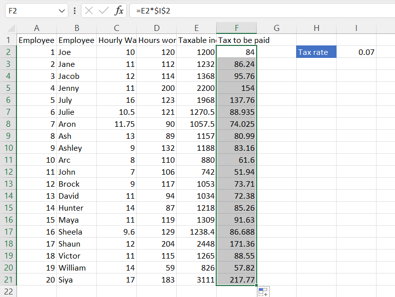
You can also utilize the autofill handle functionality to calculate the total salary for other employees.
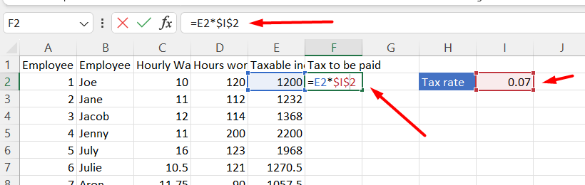
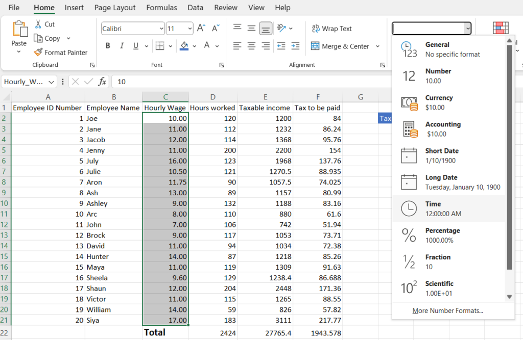
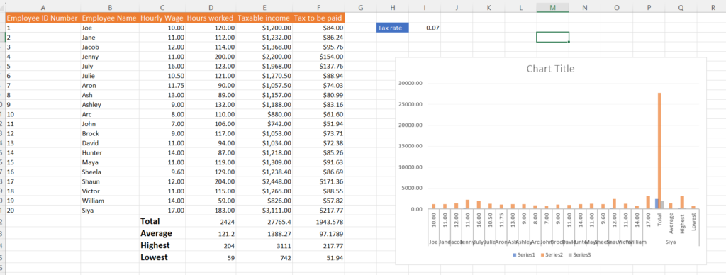
You can also calculate taxes using a formula. For instance, if the tax rate is 7 per cent, you need to enter 0.07 (representing 7%) into a cell and then create a formula. Since the tax rate remains constant for each employee, it’s important to make this value absolute. To do so, simply add a $ sign before both the row and column references. This ensures that the formula doesn’t change when copied to other cells. Additionally, you can easily edit the formula in the formula box for further customization. Once you’ve added the formula, then press Enter.
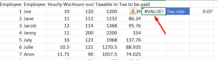
When you input an incorrect formula, Excel will display an error message. This indicates that you need to modify the formula to achieve the desired and accurate result.
In this formula, I multiply the income cell with the employee name, which is obviously wrong, and that’s why the error message is showing.
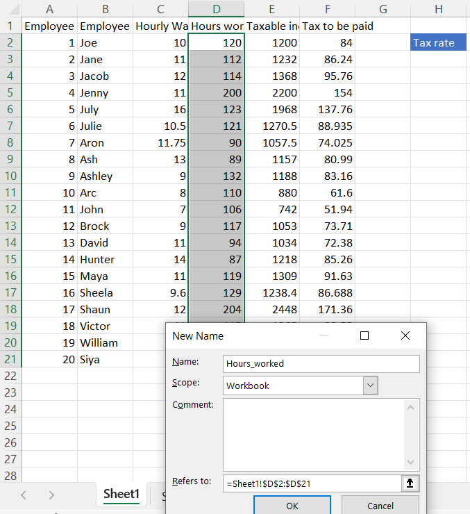
You can also assign a special name to the range, which can be very useful. This will help you with calculations and make the process faster and simpler.
By understanding and applying basic formulas, you can efficiently perform calculations and analyze data within Excel, enhancing your proficiency and productivity with the software.
4) Functions in Excel
Functions and formulas play crucial roles in Excel, though they’re not the same. Let’s delve into their distinctions and how to use them effectively.
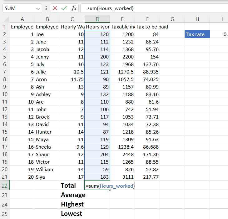
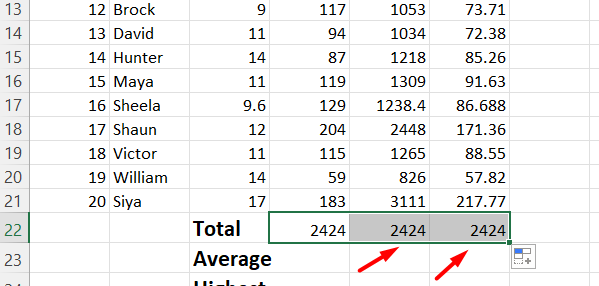
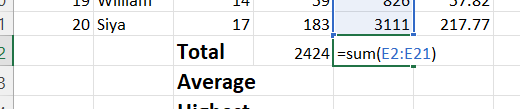
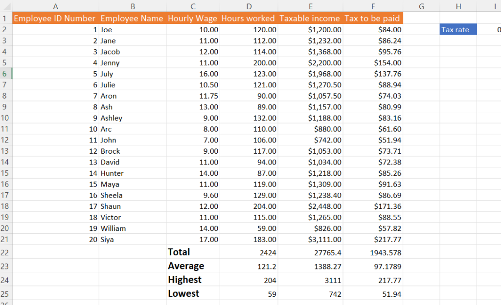
When you want to calculate the sum of data in a specific column, simply navigate to the bottom of the page and enter the equal sign (=). Then, type “sum” and you’ll see the “sum” option appear, which adds the numbers within the specified range. Here, I use the name of the range that we have given in the SUM function to calculate the sum of the range. We can’t copy the formula using the autofill function since it will sum the range of hours worked.
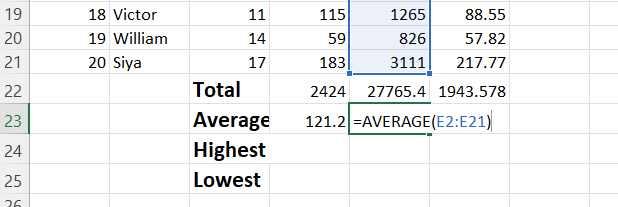
For instance, to find the average salary, you can employ the average function: =AVERAGE(E2:E21).
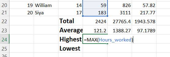
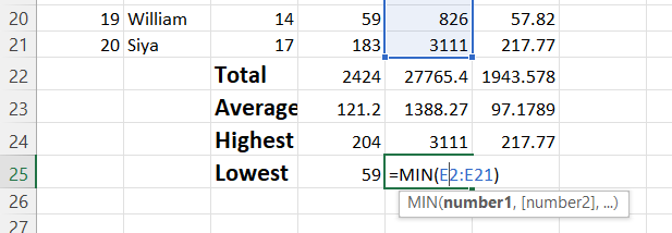
Similarly, you can determine the highest value in a range using the MAX function and the lowest value with the MIN function.
Average
Maximum
Minimum
By mastering these basic functions and understanding their distinctions, you can efficiently perform calculations and streamline your data analysis processes in Excel.
5) Formatting in Excel
Improving Data Visibility with Headings and Cell Size Adjustment
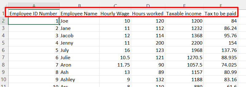
To enhance the clarity and comprehension of your data, it’s advisable to add headings. You can do this by adding an extra row above your data and naming each column accordingly. For example, you could include headings such as “Employee ID,” “Employee Name,” “Employee Hourly Wage,” and so on. Once you’ve labelled each column, make sure to bold the text to distinguish it from the rest of the data. This simple formatting technique helps organize your data and makes it easier to understand at a glance.
Sometimes, data in a cell is not fully visible because the width or height of cells in a row or column is not right. To fix this, you can hover over the row or column heading, then left-click and drag the mouse to adjust the width of the cell. This ensures your data is displayed accurately within each cell. Alternatively, for a quicker method, select all columns by clicking the column headers. Then, double-click between any two column headers. Excel will automatically adjust the size of each column to fit the content comfortably. This saves time and ensures your data remains neatly organized and easily readable.
Formatting tools
To enhance the clarity and understanding of your data, it’s essential to use correct formatting. This can be easily done by selecting the column where you want to apply formatting and clicking on the formatting button located in the ribbon. From there, you can choose the appropriate formatting options. For instance, you can select currency or accounting formats for monetary data like hourly wage, total income, and tax amounts.
Additionally, formatting options allow you to make text bold, change alignment, and modify background colors. To apply formatting to other cells, columns, or rows, simply copy the formatting of a cell or range. To do this, click on the cell or column with the desired format, then double-click on the format painter located below the paste button in the ribbon. Finally, click on the cell or range where you want to replicate the formatting.
Furthermore, Excel offers auto-formatting functions that give your data a polished appearance automatically. These features collectively ensure that your data is presented in a clear, professional, and easily understandable manner.
After selecting a formatting style for ranges
Format painter
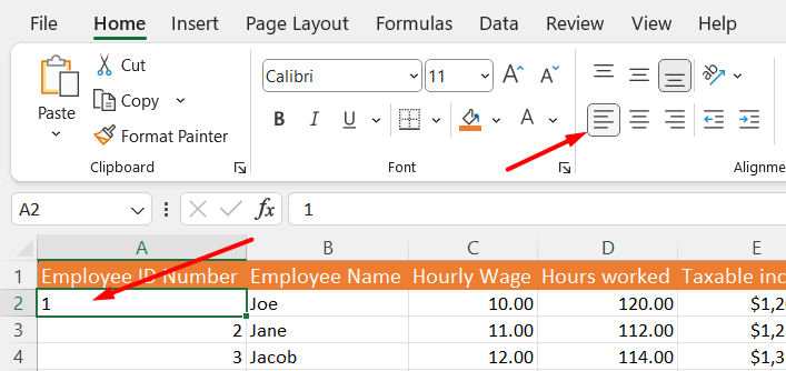
So, I want the ID numbers to start from the left side. I selected cell A2 and then changed its formatting.
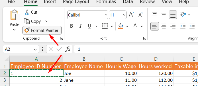
Next, I clicked on the Format Painter and used the autofill function to apply this format to the rest of the numbers in the column.
6) Charts
To present data more effectively, you can add charts to your spreadsheet. Simply select the data you wish to include in your chart, then press Alt+F1, and Excel will generate a chart for you. You can customize the chart design by clicking on the chart type and selecting the design that best fits your data.
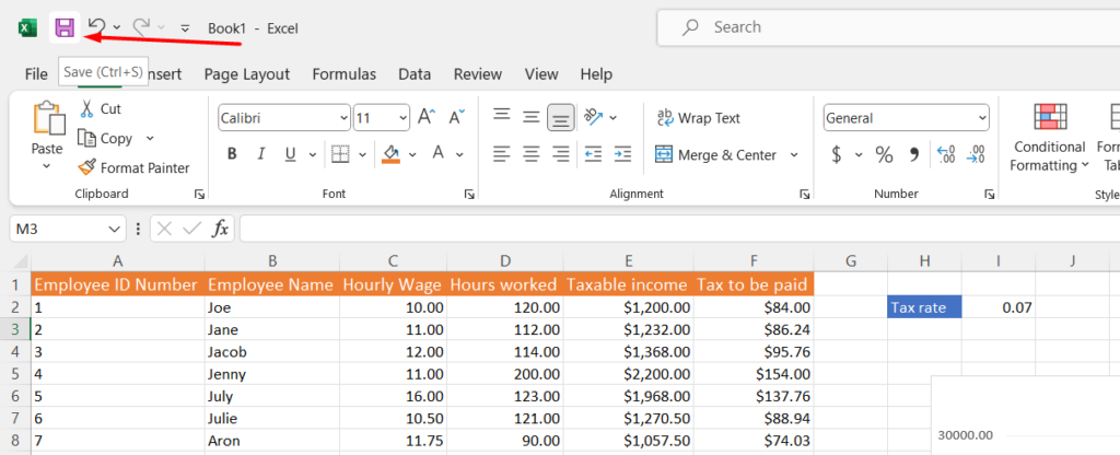
To save your workbook, simply click on the save icon.
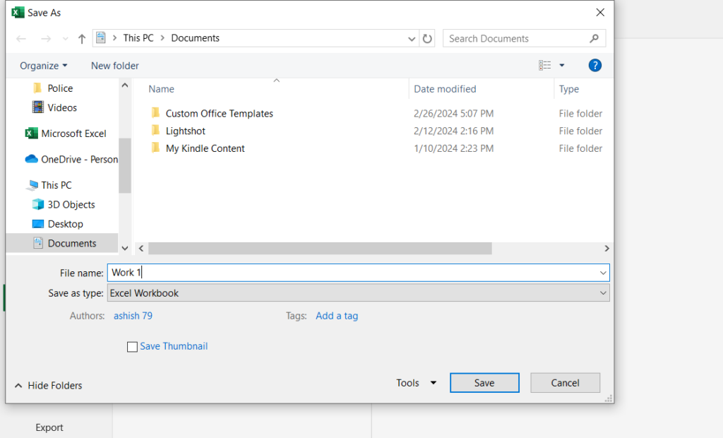
And select the ‘Recent’ option, then give your workbook a name and save it.
Conclusion
So, this covers the basics of Excel, which will help you get started and make a positive first impression. Excel skills are really important in a business setting, and if you know them, your productivity can increase multiple times. The key to improving your Excel skills is consistent practice, exploration, and watching tutorials to expand your knowledge and proficiency. It’s important to progress intelligently, focusing on mastering fundamental concepts before diving into advanced Excel techniques. Rushing into advanced topics can be overwhelming and lead to frustration, potentially causing you to lose interest. Take your time, enjoy the learning process, and gradually build your skills to avoid feeling overwhelmed or discouraged.